Give the Defnition of Limit and Continuous for a Function F R R

Point to which functions converge in analysis

${\displaystyle x}$	${\displaystyle {\frac {\sin x}{x}}}$
1	0.841471...
0.1	0.998334...
0.01	0.999983...

Although the function (sinx)/x is not defined at zero, as x becomes closer and closer to zero, (sinx)/x becomes arbitrarily close to 1. In other words, the limit of (sinx)/x, as x approaches zero, equals 1.

In mathematics, the limit of a function is a fundamental concept in calculus and analysis concerning the behavior of that function near a particular input.

Formal definitions, first devised in the early 19th century, are given below. Informally, a function f assigns an output f(x) to every input x. We say that the function has a limit L at an input p, if f(x) gets closer and closer to L as x moves closer and closer to p. More specifically, when f is applied to any input sufficiently close to p, the output value is forced arbitrarily close to L. On the other hand, if some inputs very close to p are taken to outputs that stay a fixed distance apart, then we say the limit does not exist.

The notion of a limit has many applications in modern calculus. In particular, the many definitions of continuity employ the concept of limit: roughly, a function is continuous if all of its limits agree with the values of the function. The concept of limit also appears in the definition of the derivative: in the calculus of one variable, this is the limiting value of the slope of secant lines to the graph of a function.

History [edit]

Although implicit in the development of calculus of the 17th and 18th centuries, the modern idea of the limit of a function goes back to Bolzano who, in 1817, introduced the basics of the epsilon-delta technique to define continuous functions. However, his work was not known during his lifetime.^[1]

In his 1821 book Cours d'analyse, Cauchy discussed variable quantities, infinitesimals and limits, and defined continuity of ${\displaystyle y=f(x)}$ by saying that an infinitesimal change in x necessarily produces an infinitesimal change in y, while (Grabiner 1983) claims that he used a rigorous epsilon-delta definition in proofs.^[2] In 1861, Weierstrass first introduced the epsilon-delta definition of limit in the form it is usually written today.^[3] He also introduced the notations lim and lim _{x→x 0} .^[4]

The modern notation of placing the arrow below the limit symbol is due to Hardy, which is introduced in his book A Course of Pure Mathematics in 1908.^[5]

Motivation [edit]

Imagine a person walking over a landscape represented by the graph of y = f(x). Their horizontal position is measured by the value of x, much like the position given by a map of the land or by a global positioning system. Their altitude is given by the coordinate y. They walk toward the horizontal position given by x = p. As they get closer and closer to it, they notice that their altitude approaches L. If asked about the altitude of x = p, they would then answer L.

What, then, does it mean to say, their altitude is approaching L? It means that their altitude gets nearer and nearer to L—except for a possible small error in accuracy. For example, suppose we set a particular accuracy goal for our traveler: they must get within ten meters of L. They report back that indeed, they can get within ten vertical meters of L, since they note that when they are within fifty horizontal meters of p, their altitude is always ten meters or less from L.

The accuracy goal is then changed: can they get within one vertical meter? Yes. If they are anywhere within seven horizontal meters of p, their altitude will always remain within one meter from the target L. In summary, to say that the traveler's altitude approaches L as their horizontal position approaches p, is to say that for every target accuracy goal, however small it may be, there is some neighbourhood of p whose altitude fulfills that accuracy goal.

The initial informal statement can now be explicated:

The limit of a function f(x) as x approaches p is a number L with the following property: given any target distance from L, there is a distance from p within which the values of f(x) remain within the target distance.

In fact, this explicit statement is quite close to the formal definition of the limit of a function, with values in a topological space.

More specifically, to say that

${\displaystyle \lim _{x\to p}f(x)=L,\,}$

is to say that ƒ(x) can be made as close to L as desired, by making x close enough, but not equal, top.

The following definitions, known as (ε, δ)-definitions, are the generally accepted definitions for the limit of a function in various contexts.

Functions of a single variable [edit]

(ε, δ)-definition of limit [edit]

Suppose ${\displaystyle f:\mathbb {R} \rightarrow \mathbb {R} }$ is defined on the real line and ${\displaystyle p,L\in \mathbb {R} }$ . One would say that the limit of f, as x approaches p, is L and written

${\displaystyle \lim _{x\to p}f(x)=L,}$

or alternatively as:

${\displaystyle f(x)\to L}$ as ${\displaystyle x\to p}$ (reads " ${\displaystyle f(x)}$ tends to ${\displaystyle L}$ as ${\displaystyle x}$ tends to ${\displaystyle p}$ ")

if the following property holds:

For every real ε > 0, there exists a real δ > 0 such that for all real x, 0 < | x − p | < δ implies that | f(x) − L | < ε .^[6]

A more general definition applies for functions defined on subsets of the real line. Let (a,b) be an open interval in R, and p a point of (a,b). Let f be a real-valued function defined on all of (a,b)—except possibly at p itself. It is then said that the limit of f as x approaches p is L, if for every real ε > 0, there exists a real δ > 0 such that 0 < | x − p | < δ and x ∈ (a, b) implies that | f(x) − L | < ε .

Here, note that the value of the limit does not depend on f being defined at p, nor on the value f(p)—if it is defined.

The letters ε and δ can be understood as "error" and "distance". In fact, Cauchy used ε as an abbreviation for "error" in some of his work,^[2] though in his definition of continuity, he used an infinitesimal ${\displaystyle \alpha }$ rather than either ε or δ (see Cours d'Analyse). In these terms, the error (ε) in the measurement of the value at the limit can be made as small as desired, by reducing the distance (δ) to the limit point. As discussed below, this definition also works for functions in a more general context. The idea that δ and ε represent distances helps suggest these generalizations.

Existence and one-sided limits [edit]

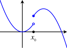
The limit as: x → x ₀ ⁺ ≠ x → x ₀ ⁻. Therefore, the limit as x → x ₀ does not exist.

Alternatively, x may approach p from above (right) or below (left), in which case the limits may be written as

${\displaystyle \lim _{x\to p^{+}}f(x)=L}$

or

${\displaystyle \lim _{x\to p^{-}}f(x)=L}$

respectively. If these limits exist at p and are equal there, then this can be referred to as the limit of f(x) at p .^[7] If the one-sided limits exist at p, but are unequal, then there is no limit at p (i.e., the limit at p does not exist). If either one-sided limit does not exist at p, then the limit at p also does not exist.

A formal definition is as follows. The limit of f(x) as x approaches p from above is L if, for every ε > 0, there exists a δ > 0 such that |f(x) −L| <ε whenever 0 <x −p <δ. The limit of f(x) as x approaches p from below is L if, for every ε > 0, there exists a δ > 0 such that |f(x) −L| <ε whenever 0 <p −x <δ.

If the limit does not exist, then the oscillation of f at p is non-zero.

More general subsets [edit]

Apart from open intervals, limits can be defined for functions on arbitrary subsets of R, as follows (Bartle & Sherbert 2000) harv error: no target: CITEREFBartleSherbert2000 (help): let f be a real-valued function defined on a subset S of the real line. Let p be a limit point of S—that is, p is the limit of some sequence of elements of S distinct from p. The limit of f, as x approaches p from values in S, is L, if for every ε > 0 , there exists a δ > 0 such that 0 < | x − p | < δ and x ∈ S implies that | f(x) − L | < ε .

This limit is often written as:

${\displaystyle L=\lim _{\stackrel {x\to p}{x\in S}}f(x).}$

The condition that f be defined on S is that S be a subset of the domain of f. This generalization includes as special cases limits on an interval, as well as left-handed limits of real-valued functions (e.g., by taking S to be an open interval of the form ${\displaystyle (-\infty ,a)}$ ), and right-handed limits (e.g., by taking S to be an open interval of the form ${\displaystyle (a,\infty )}$ ). It also extends the notion of one-sided limits to the included endpoints of (half-)closed intervals, so the square root function f(x)=√ x can have limit 0 as x approaches 0 from above.

Deleted versus non-deleted limits [edit]

The definition of limit given here does not depend on how (or whether) f is defined at p. Bartle (1967) refers to this as a deleted limit, because it excludes the value of f at p. The corresponding non-deleted limit does depend on the value of f at p, if p is in the domain of f:

• A number L is the non-deleted limit of f as x approaches p if, for every ε > 0, there exists a δ > 0 such that |x −p | <δ and x ∈ Dm(f) implies |f(x) −L | <ε.

The definition is the same, except that the neighborhood |x −p | <δ now includes the point p, in contrast to the deleted neighborhood 0 < |x −p | <δ. This makes the definition of a non-deleted limit less general. One of the advantages of working with non-deleted limits is that they allow to state the theorem about limits of compositions without any constraints on the functions (other than the existence of their non-deleted limits) (Hubbard (2015)).

Bartle (1967) notes that although by "limit" some authors do mean this non-deleted limit, deleted limits are the most popular. For example, Apostol (1974), Courant (1924), Hardy (1921), Rudin (1964), Whittaker & Watson (1902) harvtxt error: no target: CITEREFWhittakerWatson1902 (help) all take "limit" to mean the deleted limit.

Examples [edit]

Non-existence of one-sided limit(s) [edit]

The function

${\displaystyle f(x)={\begin{cases}\sin {\frac {5}{x-1}}&{\text{ for }}x<1\\0&{\text{ for }}x=1\\{\frac {0.1}{x-1}}&{\text{ for }}x>1\end{cases}}}$

has no limit at ${\displaystyle x_{0}=1}$ (the left-hand limit does not exist due to the oscillatory nature of the sine function, and the right-hand limit does not exist due to the asymptotic behaviour of the reciprocal function), but has a limit at every other x-coordinate.

The function

${\displaystyle f(x)={\begin{cases}1&x{\text{ rational }}\\0&x{\text{ irrational }}\end{cases}}}$

(a.k.a., the Dirichlet function) has no limit at any x-coordinate.

Non-equality of one-sided limits [edit]

The function

${\displaystyle f(x)={\begin{cases}1&{\text{ for }}x<0\\2&{\text{ for }}x\geq 0\end{cases}}}$

has a limit at every non-zero x-coordinate (the limit equals 1 for negative x and equals 2 for positive x). The limit at x = 0 does not exist (the left-hand limit equals 1, whereas the right-hand limit equals 2).

Limits at only one point [edit]

The functions

${\displaystyle f(x)={\begin{cases}x&x{\text{ rational }}\\0&x{\text{ irrational }}\end{cases}}}$

and

${\displaystyle f(x)={\begin{cases}|x|&x{\text{ rational }}\\0&x{\text{ irrational }}\end{cases}}}$

both have a limit at x = 0 and it equals 0.

Limits at countably many points [edit]

The function

${\displaystyle f(x)={\begin{cases}\sin x&x{\text{ irrational }}\\1&x{\text{ rational }}\end{cases}}}$

has a limit at any x-coordinate of the form ${\displaystyle {\frac {\pi }{2}}+2n\pi }$ , where n is any integer.

Functions on metric spaces [edit]

Suppose M and N are subsets of metric spaces A and B, respectively, and f : M → N is defined between M and N, with x ∈ M, p a limit point of M and L ∈ N. It is said that the limit of f as x approaches p is L and write

${\displaystyle \lim _{x\to p}f(x)=L}$

if the following property holds:

• For every ε > 0, there exists a δ > 0 such that d _B (f(x), L) < ε for all points x∈M for which 0 <d _A (x,p) <δ.^[8]

Again, note that p need not be in the domain of f, nor does L need to be in the range of f, and even if f(p) is defined it need not be equal to L.

An alternative definition using the concept of neighbourhood is as follows:

${\displaystyle \lim _{x\to p}f(x)=L}$

if, for every neighbourhood V of L in B, there exists a neighbourhood U of p in A such that f(U ∩ M − {p}) ⊆ V.

Functions on topological spaces [edit]

Suppose X,Y are topological spaces with Y a Hausdorff space. Let p be a limit point of Ω ⊆X, and L ∈Y. For a function f : Ω → Y, it is said that the limit of f as x approaches p is L (i.e., f(x) → L as x → p) and written

${\displaystyle \lim _{x\to p}f(x)=L}$

if the following property holds:

• For every open neighborhood V of L, there exists an open neighborhood U of p such that f(U ∩ Ω − {p}) ⊆ V.

This last part of the definition can also be phrased "there exists an open punctured neighbourhood U of p such that f(U∩Ω) ⊆ V ".

Note that the domain of f does not need to contain p. If it does, then the value of f at p is irrelevant to the definition of the limit. In particular, if the domain of f is X − {p} (or all of X), then the limit of f as x → p exists and is equal to L if, for all subsets Ω of X with limit point p, the limit of the restriction of f to Ω exists and is equal to L. Sometimes this criterion is used to establish the non-existence of the two-sided limit of a function on R by showing that the one-sided limits either fail to exist or do not agree. Such a view is fundamental in the field of general topology, where limits and continuity at a point are defined in terms of special families of subsets, called filters, or generalized sequences known as nets.

Alternatively, the requirement that Y be a Hausdorff space can be relaxed to the assumption that Y be a general topological space, but then the limit of a function may not be unique. In particular, one can no longer talk about the limit of a function at a point, but rather a limit or the set of limits at a point.

A function is continuous at a limit point p of and in its domain if and only if f(p) is the (or, in the general case, a) limit of f(x) as x tends to p.

Limits involving infinity [edit]

Limits at infinity [edit]

The limit of this function at infinity exists.

Let ${\displaystyle S\subseteq \mathbb {R} }$ , ${\displaystyle x\in S}$ and ${\displaystyle f:S\mapsto \mathbb {R} }$ .

The limit of f as x approaches infinity is L , denoted

${\displaystyle \lim _{x\to \infty }f(x)=L,}$

means that for all ${\displaystyle \varepsilon >0}$ , there exists c such that ${\displaystyle |f(x)-L|<\varepsilon }$ whenever x >c. Or, symbolically:

${\displaystyle \forall \varepsilon >0\;\exists c\;\forall x>c:\;|f(x)-L|<\varepsilon }$ .

Similarly, the limit of f as x approaches negative infinity is L , denoted

${\displaystyle \lim _{x\to -\infty }f(x)=L,}$

means that for all ${\displaystyle \varepsilon >0}$ there exists c such that ${\displaystyle |f(x)-L|<\varepsilon }$ whenever x <c. Or, symbolically:

${\displaystyle \forall \varepsilon >0\;\exists c\;\forall x<c:\;|f(x)-L|<\varepsilon }$ .

For example,

${\displaystyle \lim _{x\to -\infty }e^{x}=0.\,}$

Infinite limits [edit]

For a function whose values grow without bound, the function diverges and the usual limit does not exist. However, in this case one may introduce limits with infinite values. Let ${\displaystyle S\subseteq \mathbb {R} }$ , ${\displaystyle x\in S}$ and ${\displaystyle f:S\mapsto \mathbb {R} }$ . The statement the limit of f as x approaches a is infinity, denoted

${\displaystyle \lim _{x\to a}f(x)=\infty ,}$

means that for all ${\displaystyle N>0}$ there exists ${\displaystyle \delta >0}$ such that ${\displaystyle f(x)>N}$ whenever ${\displaystyle 0<|x-a|<\delta .}$

These ideas can be combined in a natural way to produce definitions for different combinations, such as

${\displaystyle \lim _{x\to \infty }f(x)=\infty ,\lim _{x\to a^{+}}f(x)=-\infty .}$

For example,

${\displaystyle \lim _{x\to 0^{+}}\ln x=-\infty .}$

Limits involving infinity are connected with the concept of asymptotes.

These notions of a limit attempt to provide a metric space interpretation to limits at infinity. In fact, they are consistent with the topological space definition of limit if

• a neighborhood of −∞ is defined to contain an interval [−∞,c) for some c ∈R,
• a neighborhood of ∞ is defined to contain an interval (c, ∞] where c ∈R, and
• a neighborhood of a ∈ R is defined in the normal way metric space R.

In this case, R is a topological space and any function of the form f:X →Y with X,Y⊆ R is subject to the topological definition of a limit. Note that with this topological definition, it is easy to define infinite limits at finite points, which have not been defined above in the metric sense.

Alternative notation [edit]

Many authors^[9] allow for the projectively extended real line to be used as a way to include infinite values as well as extended real line. With this notation, the extended real line is given as R ∪ {−∞, +∞} and the projectively extended real line is R ∪ {∞} where a neighborhood of ∞ is a set of the form {x: | x | > c}. The advantage is that one only needs three definitions for limits (left, right, and central) to cover all the cases. As presented above, for a completely rigorous account, we would need to consider 15 separate cases for each combination of infinities (five directions: −∞, left, central, right, and +∞; three bounds: −∞, finite, or +∞). There are also noteworthy pitfalls. For example, when working with the extended real line, ${\displaystyle x^{-1}}$ does not possess a central limit (which is normal):

${\displaystyle \lim _{x\to 0^{+}}{1 \over x}=+\infty ,\lim _{x\to 0^{-}}{1 \over x}=-\infty .}$

In contrast, when working with the projective real line, infinities (much like 0) are unsigned, so, the central limit does exist in that context:

${\displaystyle \lim _{x\to 0^{+}}{1 \over x}=\lim _{x\to 0^{-}}{1 \over x}=\lim _{x\to 0}{1 \over x}=\infty .}$

In fact there are a plethora of conflicting formal systems in use. In certain applications of numerical differentiation and integration, it is, for example, convenient to have signed zeroes. A simple reason has to do with the converse of ${\displaystyle \lim _{x\to 0^{-}}{x^{-1}}=-\infty }$ , namely, it is convenient for ${\displaystyle \lim _{x\to -\infty }{x^{-1}}=-0}$ to be considered true. Such zeroes can be seen as an approximation to infinitesimals.

Limits at infinity for rational functions [edit]

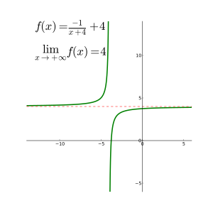
Horizontal asymptote about y = 4

There are three basic rules for evaluating limits at infinity for a rational function f(x) = p(x)/q(x): (where p and q are polynomials):

• If the degree of p is greater than the degree of q, then the limit is positive or negative infinity depending on the signs of the leading coefficients;
• If the degree of p and q are equal, the limit is the leading coefficient of p divided by the leading coefficient of q;
• If the degree of p is less than the degree of q, the limit is 0.

If the limit at infinity exists, it represents a horizontal asymptote at y = L. Polynomials do not have horizontal asymptotes; such asymptotes may however occur with rational functions.

Functions of more than one variable [edit]

By noting that |x −p| represents a distance, the definition of a limit can be extended to functions of more than one variable. In the case of a function f : R ² → R,

${\displaystyle \lim _{(x,y)\to (p,q)}f(x,y)=L}$

if

for every ε > 0 there exists a δ > 0 such that for all (x,y) with 0 < ||(x,y) − (p,q)|| < δ, then |f(x,y) −L| < ε

where ||(x,y) − (p,q)|| represents a distance defined by a norm. This can be extended to any number of variables.

Sequential limits [edit]

Let f : X → Y be a mapping from a topological space X into a Hausdorff space Y, p ∈ X a limit point of X and L ∈ Y .

The sequential limit of f as x tends to p is L if, for every sequence (x _n ) in X − {p} that converges to p, the sequence f(x _n ) converges to L.

If L is the limit (in the sense above) of f as x approaches p, then it is a sequential limit as well, however the converse need not hold in general. If in addition X is metrizable, then L is the sequential limit of f as x approaches p if and only if it is the limit (in the sense above) of f as x approaches p.

Other characterizations [edit]

In terms of sequences [edit]

For functions on the real line, one way to define the limit of a function is in terms of the limit of sequences. (This definition is usually attributed to Eduard Heine.) In this setting:

${\displaystyle \lim _{x\to a}f(x)=L}$

if, and only if, for all sequences ${\displaystyle x_{n}}$ (with ${\displaystyle x_{n}}$ not equal to a for all n) converging to ${\displaystyle a}$ the sequence ${\displaystyle f(x_{n})}$ converges to ${\displaystyle L}$ . It was shown by Sierpiński in 1916 that proving the equivalence of this definition and the definition above, requires and is equivalent to a weak form of the axiom of choice. Note that defining what it means for a sequence ${\displaystyle x_{n}}$ to converge to ${\displaystyle a}$ requires the epsilon, delta method.

Similarly as it was the case of Weierstrass's definition, a more general Heine definition applies to functions defined on subsets of the real line. Let f be a real-valued function with the domain Dm(f). Let a be the limit of a sequence of elements of Dm(f) \ {a}. Then the limit (in this sense) of f is L as x approaches p if for every sequence ${\displaystyle x_{n}}$  ∈Dm(f) \ {a} (so that for all n, ${\displaystyle x_{n}}$ is not equal to a) that converges to a, the sequence ${\displaystyle f(x_{n})}$ converges to ${\displaystyle L}$ . This is the same as the definition of a sequential limit in the preceding section obtained by regarding the subset Dm(f) of R as a metric space with the induced metric.

In non-standard calculus [edit]

In non-standard calculus the limit of a function is defined by:

${\displaystyle \lim _{x\to a}f(x)=L}$

if and only if for all ${\displaystyle x\in \mathbb {R} ^{*}}$ , ${\displaystyle f^{*}(x)-L}$ is infinitesimal whenever ${\displaystyle x-a}$ is infinitesimal. Here ${\displaystyle \mathbb {R} ^{*}}$ are the hyperreal numbers and ${\displaystyle f^{*}}$ is the natural extension of f to the non-standard real numbers. Keisler proved that such a hyperreal definition of limit reduces the quantifier complexity by two quantifiers.^[10] On the other hand, Hrbacek writes that for the definitions to be valid for all hyperreal numbers they must implicitly be grounded in the ε-δ method, and claims that, from the pedagogical point of view, the hope that non-standard calculus could be done without ε-δ methods cannot be realized in full.^[11] Bŀaszczyk et al. detail the usefulness of microcontinuity in developing a transparent definition of uniform continuity, and characterize Hrbacek's criticism as a "dubious lament".^[12]

In terms of nearness [edit]

At the 1908 international congress of mathematics F. Riesz introduced an alternate way defining limits and continuity in concept called "nearness".^[13] A point ${\displaystyle x}$ is defined to be near a set ${\displaystyle A\subseteq \mathbb {R} }$ if for every ${\displaystyle r>0}$ there is a point ${\displaystyle a\in A}$ so that ${\displaystyle |x-a|<r}$ . In this setting the

${\displaystyle \lim _{x\to a}f(x)=L}$

if and only if for all ${\displaystyle A\subseteq \mathbb {R} }$ , ${\displaystyle L}$ is near ${\displaystyle f(A)}$ whenever ${\displaystyle a}$ is near ${\displaystyle A}$ . Here ${\displaystyle f(A)}$ is the set ${\displaystyle \{f(x)|x\in A\}}$ . This definition can also be extended to metric and topological spaces.

Relationship to continuity [edit]

The notion of the limit of a function is very closely related to the concept of continuity. A function ƒ is said to be continuous at c if it is both defined at c and its value at c equals the limit of f as x approaches c:

${\displaystyle \lim _{x\to c}f(x)=f(c).}$

(We have here assumed that c is a limit point of the domain of f.)

Properties [edit]

If a function f is real-valued, then the limit of f at p is L if and only if both the right-handed limit and left-handed limit of f at p exist and are equal to L.

The function f is continuous at p if and only if the limit of f(x) as x approaches p exists and is equal to f(p). If f : M → N is a function between metric spaces M and N, then it is equivalent that f transforms every sequence in M which converges towards p into a sequence in N which converges towards f(p).

If N is a normed vector space, then the limit operation is linear in the following sense: if the limit of f(x) as x approaches p is L and the limit of g(x) as x approaches p is P, then the limit of f(x) + g(x) as x approaches p is L + P. If a is a scalar from the base field, then the limit of af(x) as x approaches p is aL.

If f and g are real-valued (or complex-valued) functions, then taking the limit of an operation on f(x) and g(x) (e.g., ${\displaystyle f+g}$ , ${\displaystyle f-g}$ , ${\displaystyle f\times g}$ , ${\displaystyle f/g}$ , ${\displaystyle f^{g}}$ ) under certain conditions is compatible with the operation of limits of f(x) and g(x). This fact is often called the algebraic limit theorem. The main condition needed to apply the following rules is that the limits on the right-hand sides of the equations exist (in other words, these limits are finite values including 0). Additionally, the identity for division requires that the denominator on the right-hand side is non-zero (division by 0 is not defined), and the identity for exponentiation requires that the base is positive, or zero while the exponent is positive (finite).

${\displaystyle {\begin{matrix}\lim \limits _{x\to p}&(f(x)+g(x))&=&\lim \limits _{x\to p}f(x)+\lim \limits _{x\to p}g(x)\\\lim \limits _{x\to p}&(f(x)-g(x))&=&\lim \limits _{x\to p}f(x)-\lim \limits _{x\to p}g(x)\\\lim \limits _{x\to p}&(f(x)\cdot g(x))&=&\lim \limits _{x\to p}f(x)\cdot \lim \limits _{x\to p}g(x)\\\lim \limits _{x\to p}&(f(x)/g(x))&=&{\lim \limits _{x\to p}f(x)/\lim \limits _{x\to p}g(x)}\\\lim \limits _{x\to p}&f(x)^{g(x)}&=&{\lim \limits _{x\to p}f(x)^{\lim \limits _{x\to p}g(x)}}\end{matrix}}}$

These rules are also valid for one-sided limits, including when p is ∞ or −∞. In each rule above, when one of the limits on the right is ∞ or −∞, the limit on the left may sometimes still be determined by the following rules.

• q + ∞ = ∞ if q ≠ −∞
• q × ∞ = ∞ if q > 0
• q × ∞ = −∞ if q < 0
• q / ∞ = 0 if q ≠ ∞ and q ≠ −∞
• ∞ ^q = 0 if q < 0
• ∞ ^q = ∞ if q > 0
• q ^∞ = 0 if 0 < q < 1
• q ^∞ = ∞ if q > 1
• q ^−∞ = ∞ if 0 < q < 1
• q ^−∞ = 0 if q > 1

(see also Extended real number line).

In other cases the limit on the left may still exist, although the right-hand side, called an indeterminate form, does not allow one to determine the result. This depends on the functions f and g. These indeterminate forms are:

• 0 / 0
• ±∞ / ±∞
• 0 × ±∞
• ∞ + −∞
• 0⁰
• ∞⁰
• 1^±∞

See further L'Hôpital's rule below and Indeterminate form.

Limits of compositions of functions [edit]

In general, from knowing that

${\displaystyle \lim _{y\to b}f(y)=c}$ and ${\displaystyle \lim _{x\to a}g(x)=b}$ ,

it does not follow that ${\displaystyle \lim _{x\to a}f(g(x))=c}$ . However, this "chain rule" does hold if one of the following additional conditions holds:

As an example of this phenomenon, consider the following function that violates both additional restrictions:

${\displaystyle f(x)=g(x)={\begin{cases}0&{\text{if }}x\neq 0\\1&{\text{if }}x=0\end{cases}}.}$

Since the value at f(0) is a removable discontinuity,

${\displaystyle \lim _{x\to a}f(x)=0}$ for all ${\displaystyle a}$ .

Thus, the naïve chain rule would suggest that the limit of f(f(x)) is 0. However, it is the case that

${\displaystyle f(f(x))={\begin{cases}1&{\text{if }}x\neq 0\\0&{\text{if }}x=0\end{cases}}}$

and so

${\displaystyle \lim _{x\to a}f(f(x))=1}$ for all ${\displaystyle a}$ .

Limits of special interest [edit]

Rational functions [edit]

For ${\displaystyle n}$ a nonnegative integer and constants ${\displaystyle a_{1},a_{2},a_{3},\ldots ,a_{n}}$ and ${\displaystyle b_{1},b_{2},b_{3},\ldots ,b_{n}}$ ,

• ${\displaystyle \lim _{x\to \infty }{\frac {a_{1}{x}^{n}+a_{2}{x}^{n-1}+a_{3}{x}^{n-2}+...+a_{n}}{b_{1}{x}^{n}+b_{2}{x}^{n-1}+b_{3}{x}^{n-2}+...+b_{n}}}={\frac {a_{1}}{b_{1}}}}$

This can be proven by dividing both the numerator and denominator by ${\displaystyle x^{n}}$ . If the numerator is a polynomial of higher degree, the limit does not exist. If the denominator is of higher degree, the limit is 0.

Trigonometric functions [edit]

Exponential functions [edit]

Logarithmic functions [edit]

L'Hôpital's rule [edit]

This rule uses derivatives to find limits of indeterminate forms 0/0 or ±∞/∞, and only applies to such cases. Other indeterminate forms may be manipulated into this form. Given two functions f(x) and g(x), defined over an open interval I containing the desired limit point c, then if:

1. ${\displaystyle \lim _{x\to c}f(x)=\lim _{x\to c}g(x)=0,}$ or ${\displaystyle \lim _{x\to c}f(x)=\pm \lim _{x\to c}g(x)=\pm \infty }$ , and
2. ${\displaystyle f}$ and ${\displaystyle g}$ are differentiable over ${\displaystyle I\setminus \{c\}}$ , and
3. ${\displaystyle g'(x)\neq 0}$ for all ${\displaystyle x\in I\setminus \{c\}}$ , and
4. ${\displaystyle \lim _{x\to c}{\frac {f'(x)}{g'(x)}}}$ exists,

then:

${\displaystyle \lim _{x\to c}{\frac {f(x)}{g(x)}}=\lim _{x\to c}{\frac {f'(x)}{g'(x)}}}$

Normally, the first condition is the most important one.

For example: ${\displaystyle \lim _{x\to 0}{\frac {\sin(2x)}{\sin(3x)}}=\lim _{x\to 0}{\frac {2\cos(2x)}{3\cos(3x)}}={\frac {2\cdot 1}{3\cdot 1}}={\frac {2}{3}}.}$

Summations and integrals [edit]

Specifying an infinite bound on a summation or integral is a common shorthand for specifying a limit.

A short way to write the limit ${\displaystyle \lim _{n\to \infty }\sum _{i=s}^{n}f(i)}$ is ${\displaystyle \sum _{i=s}^{\infty }f(i)}$ . An important example of limits of sums such as these are series.

A short way to write the limit ${\displaystyle \lim _{x\to \infty }\int _{a}^{x}f(t)\;dt}$ is ${\displaystyle \int _{a}^{\infty }f(t)\;dt}$ .

A short way to write the limit ${\displaystyle \lim _{x\to -\infty }\int _{x}^{b}f(t)\;dt}$ is ${\displaystyle \int _{-\infty }^{b}f(t)\;dt}$ .

See also [edit]

• Big O notation – Notation describing limiting behavior
• L'Hôpital's rule – Mathematical rule for evaluating certain limits
• List of limits
• Limit of a sequence – Value to which tends an infinite sequence
• Limit superior and limit inferior
• Net (mathematics) – A generalization of a sequence of points
• Non-standard calculus
• Squeeze theorem – Method for finding limits in calculus
• Subsequential limit – The limit of some subsequence

Notes [edit]

1. ^ Felscher, Walter (2000), "Bolzano, Cauchy, Epsilon, Delta", American Mathematical Monthly, 107 (9): 844–862, doi:10.2307/2695743, JSTOR 2695743
2. ^ ^{a b} Grabiner, Judith V. (1983), "Who Gave You the Epsilon? Cauchy and the Origins of Rigorous Calculus", American Mathematical Monthly, 90 (3): 185–194, doi:10.2307/2975545, JSTOR 2975545 , collected in Who Gave You the Epsilon?, ISBN 978-0-88385-569-0 pp. 5–13. Also available at: http://www.maa.org/pubs/Calc_articles/ma002.pdf
3. ^ Sinkevich, G. I. (2017). "Historia epsylontyki" (PDF). Antiquitates Mathematicae. Cornell University. 10. arXiv:1502.06942. doi:10.14708/am.v10i0.805. Retrieved 19 October 2021.
4. ^ Burton, David M. (1997), The History of Mathematics: An introduction (Third ed.), New York: McGraw–Hill, pp. 558–559, ISBN978-0-07-009465-9
5. ^ Miller, Jeff (1 December 2004), Earliest Uses of Symbols of Calculus , retrieved 18 December 2008
6. ^ Weisstein, Eric W. "Epsilon-Delta Definition". mathworld.wolfram.com . Retrieved 18 August 2020.
7. ^ Weisstein, Eric W. "Limit". mathworld.wolfram.com . Retrieved 18 August 2020.
8. ^ Rudin, W (1986). Principles of mathematical analysis. McGraw - Hill Book C. p. 84. OCLC 962920758.
9. ^ For example, Limit at Encyclopedia of Mathematics
10. ^ Keisler, H. Jerome (2008), "Quantifiers in limits" (PDF), Andrzej Mostowski and foundational studies, IOS, Amsterdam, pp. 151–170
11. ^ Hrbacek, K. (2007), "Stratified Analysis?", in Van Den Berg, I.; Neves, V. (eds.), The Strength of Nonstandard Analysis, Springer
12. ^ Bŀaszczyk, Piotr; Katz, Mikhail; Sherry, David (2012), "Ten misconceptions from the history of analysis and their debunking", Foundations of Science, 18 (1): 43–74, arXiv:1202.4153, doi:10.1007/s10699-012-9285-8, S2CID 119134151
13. ^ F. Riesz (7 April 1908), "Stetigkeitsbegriff und abstrakte Mengenlehre (The Concept of Continuity and Abstract Set Theory)", 1908 International Congress of Mathematicians

References [edit]

• Apostol, Tom M. (1974), Mathematical Analysis (2 ed.), Addison–Wesley, ISBN0-201-00288-4
• Bartle, Robert (1967), The elements of real analysis, Wiley
• Courant, Richard (1924), Vorlesungen über Differential- und Integralrechnung, Springer Verlag
• Hardy, G.H. (1921), A course in pure mathematics, Cambridge University Press
• Hubbard, John H. (2015), Vector calculus, linear algebra, and differential forms: A unified approach (Fifth ed.), Matrix Editions
• Page, Warren; Hersh, Reuben; Selden, Annie; et al., eds. (2002), "Media Highlights", The College Mathematics, 33 (2): 147–154, JSTOR 2687124 .
• Rudin, Walter (1964), Principles of mathematical analysis, McGraw-Hill
• Sutherland, W. A. (1975), Introduction to Metric and Topological Spaces, Oxford: Oxford University Press, ISBN0-19-853161-3
• Sherbert, Robert (2000), Introduction to real analysis, Wiley
• Whittaker; Watson (1904), A Course of Modern Analysis, Cambridge University Press

External links [edit]

• MacTutor History of Weierstrass.
• MacTutor History of Bolzano
• Visual Calculus by Lawrence S. Husch, University of Tennessee (2001)

burnsbeforning.blogspot.com

Source: https://en.wikipedia.org/wiki/Limit_of_a_function

Share this post